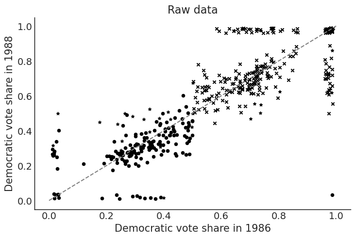
4 Regression and Other Stories: Congress

Farhan Reynaldo

Nov 12th, 2021

from pathlib import Path

import arviz as az
import bambi as bmb
import matplotlib.pyplot as plt
import numpy as np
import pandas as pd

DATA_PATH = Path("../../data")

rng = np.random.default_rng(seed=12)
az.style.use("arviz-white")

congress = pd.read_csv(DATA_PATH / "congress.csv")
congress.head()

	inc86	inc88	inc90	v86	v88	v90	v86_adj	v88_adj	v90_adj
0	1	1	1	0.745036	0.772443	0.714029	0.745036	0.772443	0.714029
1	1	1	1	0.673845	0.636182	0.597050	0.673845	0.636182	0.597050
2	1	1	0	0.696457	0.664928	0.521043	0.696457	0.664928	0.521043
3	-1	-1	-1	0.464590	0.273834	0.234377	0.464590	0.273834	0.234377
4	-1	-1	0	0.391095	0.263613	0.477439	0.391095	0.263613	0.477439

4.1 Regression predicting 1988 from 1986

data88 = pd.DataFrame(
    dict(
        vote=congress["v88_adj"],
        past_vote=congress["v86_adj"],
        inc=congress["inc88"],
    )
)

model_88 = bmb.Model("vote ~ past_vote + inc", data=data88)
idata_88 = model_88.fit()
az.summary(idata_88, kind="stats")

100.00% [8000/8000 00:09<00:00 Sampling 4 chains, 0 divergences]

	mean	sd	hdi_3%	hdi_97%
Intercept	0.238	0.017	0.204	0.269
past_vote	0.520	0.033	0.459	0.582
inc	0.097	0.007	0.084	0.109
vote_sigma	0.067	0.002	0.063	0.072

4.2 Simulation for inferences and predictions of new data points

4.2.1 Predict from 1988 to 1990

data90 = pd.DataFrame(
    dict(
        past_vote=congress["v88_adj"],
        inc=congress["inc90"],
    )
)

4.2.2 Simulate predictive simulations of the vector of new outcomes

pred90 = model_88.predict(idata_88, data=data90, kind="pps", inplace=False)

4.2.3 Simulate the number of elections predicted to be won by the Democrats in 1990

dems_pred = pred90.posterior_predictive["vote"].values.reshape(-1, 435)
dems_pred = (dems_pred > 0.5).sum(axis=1)

4.2.4 Our posterior mean and sd of how many districts the Dems will win

print(f"mean: {dems_pred.mean():.1f}, std: {dems_pred.std():.1f}")

mean: 260.0, std: 2.5

4.2.5 Histogram of how many districts the Dems will win

plt.hist(dems_pred, color="gray");

4.3 Graphs

v88_hist = np.where(
    congress["v88"] < 0.1,
    0.0001,
    np.where(congress["v88"] > 0.9, 0.9999, congress["v88"]),
)

fig, ax = plt.subplots()
ax.hist(v88_hist, color="gray", bins=np.arange(0, 1.05, 0.05))
ax.set_xlabel("Democratic share of the two-party vote")
ax.set_title("Congressional elections in 1988");

def jitt(vote):
    n = len(vote)
    return np.where(
        vote < 0.1,
        rng.uniform(0.01, 0.04, n),
        np.where(vote > 0.9, rng.uniform(0.96, 0.99, n), vote),
    )


j_v86 = jitt(congress["v86"])
j_v88 = jitt(congress["v88"])

fig, ax = plt.subplots()
ax.scatter(
    j_v86[congress["inc88"] == 0],
    j_v88[congress["inc88"] == 0],
    marker="*",
    c="black",
    s=20,
)
ax.scatter(
    j_v86[congress["inc88"] == 1],
    j_v88[congress["inc88"] == 1],
    marker="x",
    c="black",
    s=20,
)
ax.scatter(
    j_v86[congress["inc88"] == -1],
    j_v88[congress["inc88"] == -1],
    marker="o",
    c="black",
    s=20,
)
ax.plot([0, 1], [0, 1], color="gray", linestyle="--")

ax.set_title("Raw data")
ax.set_xlabel("Democratic vote share in 1986")
ax.set_ylabel("Democratic vote share in 1988")

Text(0, 0.5, 'Democratic vote share in 1988')

fig, ax = plt.subplots()
ax.plot([0, 1], [0, 1], color="gray", linestyle="--")
ax.set_xlabel("Democratic vote share in 1986")
ax.set_ylabel("Democratic vote share in 1988")
ax.scatter(
    congress["v86_adj"][congress["inc88"] == 0],
    congress["v88_adj"][congress["inc88"] == 0],
    marker="*",
    c="black",
    s=20,
)
ax.scatter(
    congress["v86_adj"][congress["inc88"] == 1],
    congress["v88_adj"][congress["inc88"] == 1],
    marker="x",
    c="black",
    s=20,
)
ax.scatter(
    congress["v86_adj"][congress["inc88"] == -1],
    congress["v88_adj"][congress["inc88"] == -1],
    marker="o",
    c="black",
    s=20,
)
ax.set_title("Adjusted data")

Text(0.5, 1.0, 'Adjusted data')