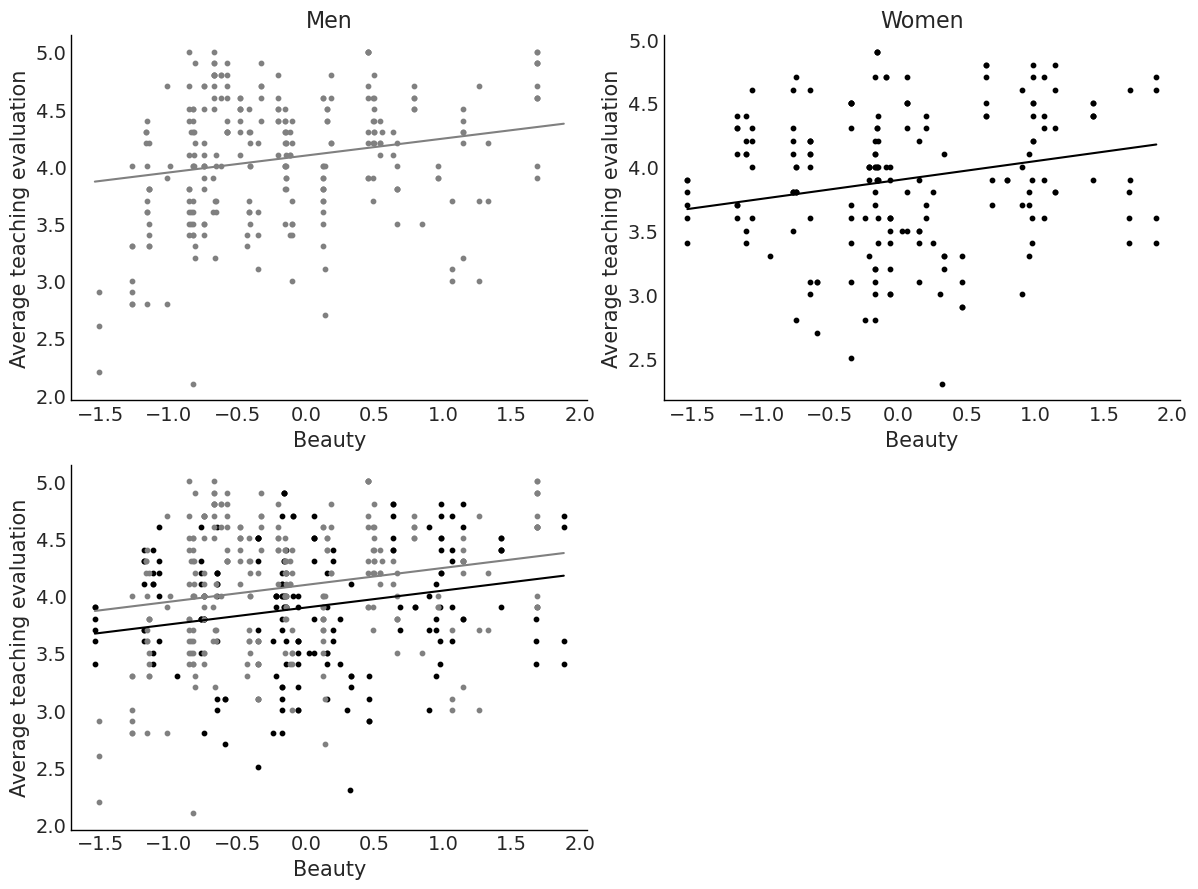
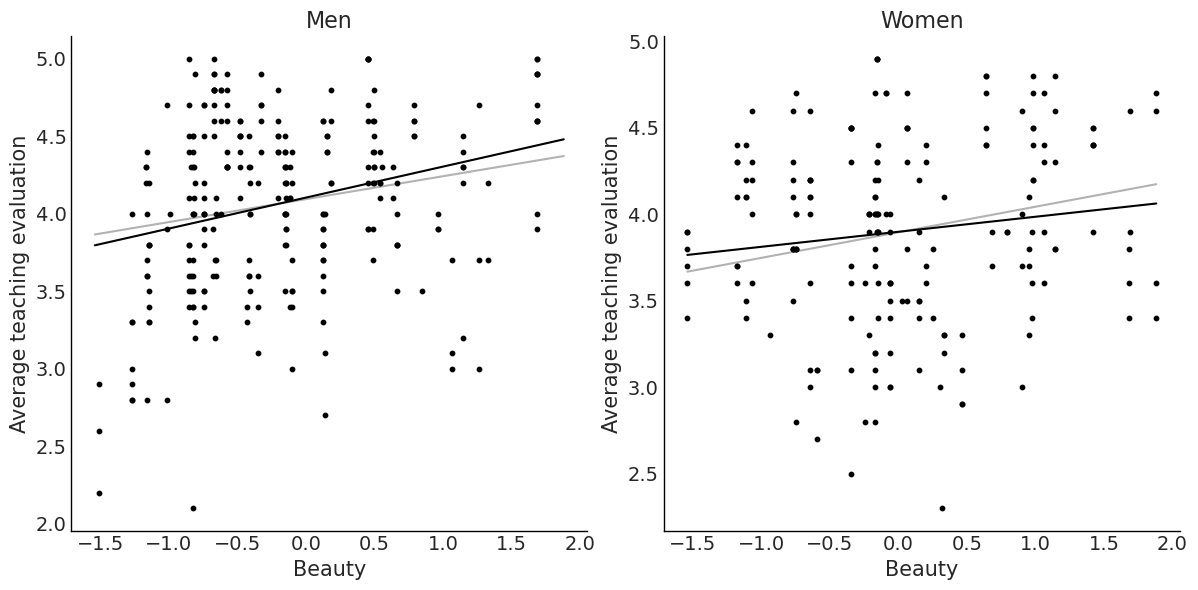
3  Regression and Other Stories: Beauty and Teaching Quality

Farhan Reynaldo

Nov 11th, 2021

from pathlib import Path

import arviz as az
import bambi as bmb
import matplotlib.pyplot as plt
import numpy as np
import pandas as pd

DATA_PATH = Path("../../data")
az.style.use("arviz-white")
beauty = pd.read_csv(DATA_PATH / "beauty.csv")
beauty.head()
eval beauty female age minority nonenglish lower course_id
0 4.3 0.201567 1 36 1 0 0 3
1 4.5 -0.826081 0 59 0 0 0 0
2 3.7 -0.660333 0 51 0 0 0 4
3 4.3 -0.766312 1 40 0 0 0 2
4 4.4 1.421445 1 31 0 0 0 0

3.1 Do more beautiful profs get higher evaluations?

3.1.1 Make a scatterplot of data

fig, ax = plt.subplots()
ax.scatter("beauty", "eval", data=beauty, color="black", s=10, alpha=0.7);

3.1.2 Fit a linear regression

model_1 = bmb.Model("eval ~ beauty", data=beauty)
idata_1 = model_1.fit()
az.summary(idata_1, kind="stats")
100.00% [8000/8000 00:03<00:00 Sampling 4 chains, 0 divergences]
mean sd hdi_3% hdi_97%
Intercept 4.010 0.026 3.964 4.060
beauty 0.133 0.032 0.070 0.189
eval_sigma 0.547 0.019 0.514 0.584
stats_1 = az.summary(idata_1, kind="stats")["mean"]
x = np.linspace(beauty["beauty"].min(), beauty["beauty"].max(), 10)
y_pred = stats_1["Intercept"] + stats_1["beauty"] * x

fig, ax = plt.subplots()
ax.scatter("beauty", "eval", data=beauty, color="black", s=10)
ax.set_xlabel("Beauty")
ax.set_ylabel("Average teaching evaluation")
ax.plot(x, y_pred, color="black")
ax.plot(x, y_pred + stats_1["eval_sigma"], color="black", linestyle="--")
ax.plot(x, y_pred - stats_1["eval_sigma"], color="black", linestyle="--");

3.2 Do things differ for male and female profs?

3.2.1 Parallel regression lines

model_2 = bmb.Model("eval ~ beauty + female", data=beauty)
idata_2 = model_2.fit()
az.summary(idata_2, kind="stats")
100.00% [8000/8000 00:06<00:00 Sampling 4 chains, 0 divergences]
mean sd hdi_3% hdi_97%
Intercept 4.094 0.033 4.032 4.154
beauty 0.148 0.032 0.087 0.209
female -0.198 0.052 -0.295 -0.104
eval_sigma 0.538 0.018 0.506 0.573

3.2.2 Make two subplots

stats_2 = az.summary(idata_2, kind="stats")["mean"]
x = np.linspace(beauty["beauty"].min(), beauty["beauty"].max(), 10)
y_pred_male = stats_2["Intercept"] + stats_2["beauty"] * x
y_pred_female = stats_2["Intercept"] + stats_2["female"] + stats_2["beauty"] * x

fig, ((ax1, ax2), (ax3, ax4)) = plt.subplots(2, 2, figsize=(12, 9))

# Men
ax1.scatter("beauty", "eval", data=beauty.query("female == 0"), color="grey", s=10)
ax1.set_title("Men")
ax1.set_xlabel("Beauty")
ax1.set_ylabel("Average teaching evaluation")
ax1.plot(x, y_pred_male, color="grey")

# Women
ax2.scatter("beauty", "eval", data=beauty.query("female == 1"), color="black", s=10)
ax2.set_title("Women")
ax2.set_xlabel("Beauty")
ax2.set_ylabel("Average teaching evaluation")
ax2.plot(x, y_pred_female, color="black")

# Both sexes
ax3.scatter("beauty", "eval", data=beauty.query("female == 1"), color="black", s=10)
ax3.scatter("beauty", "eval", data=beauty.query("female == 0"), color="grey", s=10)
ax3.set_xlabel("Beauty")
ax3.set_ylabel("Average teaching evaluation")
ax3.plot(x, y_pred_female, color="black")
ax3.plot(x, y_pred_male, color="grey")

ax4.remove()
plt.tight_layout();

3.3 Do things differ for male and female profs?

3.3.1 Non-parallel regression lines

model_3 = bmb.Model("eval ~ beauty + female + beauty*female", data=beauty)
idata_3 = model_3.fit()
az.summary(idata_3, kind="stats")
100.00% [8000/8000 00:10<00:00 Sampling 4 chains, 0 divergences]
mean sd hdi_3% hdi_97%
Intercept 4.104 0.033 4.041 4.165
beauty 0.200 0.043 0.124 0.284
female -0.205 0.052 -0.303 -0.108
beauty:female -0.113 0.063 -0.231 0.002
eval_sigma 0.537 0.017 0.502 0.568
stats_3 = az.summary(idata_3, kind="stats")["mean"]
x = np.linspace(beauty["beauty"].min(), beauty["beauty"].max(), 10)
y_pred_male_interaction = stats_3["Intercept"] + stats_3["beauty"] * x
y_pred_female_interaction = (
    stats_3["Intercept"]
    + stats_3["female"] * 1
    + stats_3["beauty"] * x
    + stats_3["beauty:female"] * x * 1
)

fig, (ax1, ax2) = plt.subplots(1, 2, figsize=(12, 6))

# Men
ax1.scatter("beauty", "eval", data=beauty.query("female == 0"), color="black", s=10)
ax1.set_title("Men")
ax1.set_xlabel("Beauty")
ax1.set_ylabel("Average teaching evaluation")
ax1.plot(x, y_pred_male, color="black", alpha=0.3)
ax1.plot(x, y_pred_male_interaction, color="black")

# Women
ax2.scatter("beauty", "eval", data=beauty.query("female == 1"), color="black", s=10)
ax2.set_title("Women")
ax2.set_xlabel("Beauty")
ax2.set_ylabel("Average teaching evaluation")
ax2.plot(x, y_pred_female, color="black", alpha=0.3)
ax2.plot(x, y_pred_female_interaction, color="black")

plt.tight_layout();

3.4 More models

3.4.1 Add age

model_4 = bmb.Model("eval ~ beauty + female + age", data=beauty)
idata_4 = model_4.fit()
az.summary(idata_4, kind="stats")
100.00% [8000/8000 00:10<00:00 Sampling 4 chains, 0 divergences]
mean sd hdi_3% hdi_97%
Intercept 4.223 0.143 3.965 4.503
beauty 0.140 0.034 0.078 0.205
female -0.210 0.053 -0.308 -0.112
age -0.003 0.003 -0.008 0.003
eval_sigma 0.539 0.018 0.504 0.572

3.4.2 Add minority

model_5 = bmb.Model("eval ~ beauty + female + minority", data=beauty)
idata_5 = model_5.fit()
az.summary(idata_5, kind="stats")
100.00% [8000/8000 00:06<00:00 Sampling 4 chains, 0 divergences]
mean sd hdi_3% hdi_97%
Intercept 4.105 0.035 4.038 4.168
beauty 0.150 0.033 0.088 0.210
female -0.189 0.053 -0.287 -0.093
minority -0.103 0.073 -0.239 0.032
eval_sigma 0.538 0.018 0.505 0.573

3.4.3 Add nonenglish

model_6 = bmb.Model("eval ~ beauty + female + nonenglish", data=beauty)
idata_6 = model_6.fit()
az.summary(idata_6, kind="stats")
100.00% [8000/8000 00:05<00:00 Sampling 4 chains, 0 divergences]
mean sd hdi_3% hdi_97%
Intercept 4.115 0.034 4.051 4.179
beauty 0.150 0.032 0.092 0.213
female -0.198 0.052 -0.296 -0.102
nonenglish -0.334 0.103 -0.537 -0.151
eval_sigma 0.533 0.018 0.501 0.569

3.4.4 Add nonenglish and lower

model_7 = bmb.Model("eval ~ beauty + female + nonenglish + lower", data=beauty)
idata_7 = model_7.fit()
az.summary(idata_7, kind="stats")
100.00% [8000/8000 00:05<00:00 Sampling 4 chains, 0 divergences]
mean sd hdi_3% hdi_97%
Intercept 4.078 0.039 4.005 4.152
beauty 0.147 0.032 0.089 0.210
female -0.191 0.052 -0.290 -0.097
nonenglish -0.307 0.105 -0.488 -0.102
lower 0.094 0.053 -0.003 0.192
eval_sigma 0.532 0.018 0.500 0.565
## Simple model with course indicators
### Include course indicators in a regression
model_8 = bmb.Model("eval ~ beauty + C(course_id)", data=beauty)
idata_8 = model_8.fit()
az.summary(idata_8, kind="stats")
100.00% [8000/8000 00:04<00:00 Sampling 4 chains, 0 divergences]
mean sd hdi_3% hdi_97%
Intercept 4.031 0.031 3.974 4.091
beauty 0.136 0.033 0.074 0.200
C(course_id)[1] 0.364 0.239 -0.071 0.821
C(course_id)[2] 0.419 0.369 -0.268 1.106
C(course_id)[3] -0.175 0.189 -0.527 0.186
C(course_id)[4] -0.201 0.122 -0.436 0.021
C(course_id)[5] 0.017 0.254 -0.471 0.467
C(course_id)[6] -0.126 0.211 -0.546 0.253
C(course_id)[7] -0.325 0.272 -0.819 0.212
C(course_id)[8] -0.143 0.378 -0.848 0.568
C(course_id)[9] -0.427 0.187 -0.761 -0.066
C(course_id)[10] 0.421 0.234 -0.026 0.843
C(course_id)[11] -0.071 0.364 -0.707 0.656
C(course_id)[12] 0.018 0.303 -0.556 0.572
C(course_id)[13] -0.082 0.305 -0.643 0.499
C(course_id)[14] -0.512 0.308 -1.057 0.105
C(course_id)[15] -1.434 0.375 -2.093 -0.693
C(course_id)[16] 0.176 0.263 -0.313 0.690
C(course_id)[17] 0.336 0.202 -0.041 0.723
C(course_id)[18] 0.267 0.261 -0.222 0.754
C(course_id)[19] -0.309 0.220 -0.715 0.098
C(course_id)[20] 0.456 0.244 0.008 0.922
C(course_id)[21] -0.391 0.144 -0.685 -0.131
C(course_id)[22] -0.286 0.162 -0.602 0.017
C(course_id)[23] 0.372 0.236 -0.060 0.800
C(course_id)[24] -0.240 0.306 -0.823 0.333
C(course_id)[25] -0.138 0.304 -0.687 0.456
C(course_id)[26] 0.234 0.307 -0.330 0.807
C(course_id)[27] 0.132 0.369 -0.527 0.851
C(course_id)[28] 0.431 0.262 -0.088 0.909
C(course_id)[29] -0.089 0.373 -0.784 0.597
C(course_id)[30] 0.300 0.191 -0.045 0.659
eval_sigma 0.526 0.018 0.493 0.558